Clustered placement gallery (analytic vs. bootstrap)

This short gallery compares analytic and bootstrap DBH payloads under the clustered placement mode. It reuses the seeded fixture tests/fixtures/synthesis/clustered_gallery.json so plots stay reproducible across refactors.

Load the fixture and compute summary stats

from pathlib import Path
import json
import numpy as np

payload = json.loads(Path("tests/fixtures/synthesis/clustered_gallery.json").read_text())
polygon = np.asarray(payload["polygon"], dtype=float)
print(payload["analytic"]["mean_dbh"], payload["bootstrap"]["mean_dbh"])

Expected means (seed=2025, cluster_spread=0.08, min_spacing=0.05, 2×1.5 polygon):

• Analytic (lognormal μ=2.0, σ²=0.25, n=10): mean DBH ≈ 11.56 cm (σ ≈ 6.79).

• Bootstrap (empirical vectors, n=10): mean DBH ≈ 14.20 cm (σ ≈ 2.97).

Visualise clustered placement

import matplotlib.pyplot as plt
from nemora.synthesis import stands, stems

def analytic_sampler():
    entry = stands.StandBootstrapLibraryEntry(
        identifier="analytic-1",
        source="analytic",
        metadata={"distribution": "lognormal", "parameters": {"mu": 2.0, "sigma2": 0.25}, "sample_size": 10},
        dbh_vectors={},
    )
    assignment = stands.StandBootstrapAssignment(
        stand_id="stand-0001",
        vegetation_type="fir",
        age_class="60-80",
        area=4.0,
        bootstrap_id="analytic-1",
    )
    return stems.StandDBHSampler(assignment=assignment, entry=entry)

def bootstrap_sampler(vectors):
    entry = stands.StandBootstrapLibraryEntry(
        identifier="bootstrap-1",
        source="bootstrap.json",
        metadata={"distribution": "empirical", "sample_size": 10, "mode": "bootstrap"},
        dbh_vectors=vectors,
    )
    assignment = stands.StandBootstrapAssignment(
        stand_id="stand-0002",
        vegetation_type="pine",
        age_class="40-60",
        area=3.5,
        bootstrap_id="bootstrap-1",
    )
    return stems.StandDBHSampler(assignment=assignment, entry=entry)

fixture = json.loads(Path("tests/fixtures/synthesis/clustered_gallery.json").read_text())
polygon = np.asarray(fixture["polygon"], dtype=float)

rng = np.random.default_rng(fixture["analytic"]["seed"])
anal_records = stems.place_trees_with_dbh(
    polygon,
    analytic_sampler(),
    rng=rng,
    config=stems.TreePlacementConfig(mode="clustered", cluster_spread=fixture["analytic"]["cluster_spread"], min_spacing=0.05),
)

rng = np.random.default_rng(fixture["bootstrap"]["seed"])
boot_records = stems.place_trees_with_dbh(
    polygon,
    bootstrap_sampler(fixture["bootstrap"]["vectors"]),
    rng=rng,
    config=stems.TreePlacementConfig(mode="clustered", cluster_spread=fixture["bootstrap"]["cluster_spread"], min_spacing=0.05),
)

fig, ax = plt.subplots(figsize=(6, 4))
poly = np.vstack([polygon, polygon[0]])  # close ring for plotting
ax.plot(poly[:, 0], poly[:, 1], color="black", lw=1, label="polygon")

ax.scatter(
    [r["x"] for r in anal_records],
    [r["y"] for r in anal_records],
    c=[r["dbh"] for r in anal_records],
    cmap="Blues",
    marker="o",
    label="analytic",
    alpha=0.8,
)
ax.scatter(
    [r["x"] for r in boot_records],
    [r["y"] for r in boot_records],
    c=[r["dbh"] for r in boot_records],
    cmap="Oranges",
    marker="x",
    label="bootstrap",
    alpha=0.9,
)
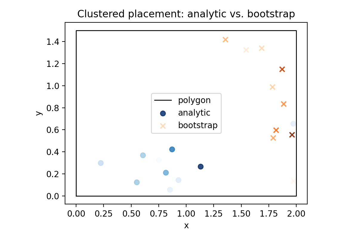
ax.set_title("Clustered placement: analytic vs. bootstrap DBH")
ax.set_xlabel("x")
ax.set_ylabel("y")
ax.legend()
ax.set_aspect("equal")
plt.tight_layout()
plt.savefig("docs/examples/clustered_gallery.png", dpi=200)

Rendered preview (placeholder coefficients):

If placement or DBH draws change, rerun the snippet and compare against the expected means from the
fixture; the regression tests (`tests/test_synthesis_stems.py::test_clustered_gallery_fixture_alignment`)
will also fail if behaviour drifts.