Fit HPS Inventories

This guide walks through fitting the horizontal point sampling (HPS) workflow using the nemora CLI and Python API. It extends the weighted estimator described in the UBC FRESH Lab manuscript and relies on the probability distributions catalogued in the distribution reference.

Prerequisites

• An HPS tally file with columns dbh_cm (bin midpoints) and tally (per-plot counts).

• The basal area factor (BAF) used during cruise design.

• Python environment with nemora installed. One approach:

python -m venv .venv
source .venv/bin/activate
pip install -e ".[dev]"

CLI Workflow

1. Inspect available distributions:

nemora registry

2. Fit the HPS inventory with the default candidate set (weibull, gamma):

nemora fit-hps data/hps_tally.csv --baf 2.0

Pass additional --distribution options to try alternative PDFs as the CLI evolves. The command prints RSS, small-sample AIC (AICc), Pearson chi-square, Kolmogorov–Smirnov, Cramér–von Mises, and Anderson–Darling statistics (plus residual summaries) for each candidate distribution so you can compare fits at a glance. Generalised secant mixtures are exposed as gsmN (for any integer N ≥ 2), so a command such as nemora fit-hps ... -d gsm3 -d gsm6 will evaluate both three- and six-component blends. Use --distribution (repeatable) to limit the candidate list and --show-parameters to include the fitted parameter estimates. For example:

nemora fit-hps data/hps_tally.csv --baf 2.0 -d weibull -d gamma --show-parameters

The grouped Weibull solver defaults to auto, which refines the least-squares seed with a Newton update and quietly falls back to the stable least-squares solution if the grouped maximum-likelihood step drifts. Use --grouped-weibull-mode ls to pin the legacy behaviour or --grouped-weibull-mode mle to require the grouped likelihood path (the command will exit with an error if the refinement fails under the forced mle mode). To stay numerically stable, the solver applies the conditional offset from the manuscript: the Weibull support is shifted by min(DBH) – 0.5 cm before evaluating grouped probabilities. Johnson SB fits now run an EM pass that updates the Beta shape parameters in grouped space, while Birnbaum–Saunders grouped fits attempt a truncated-normal EM step before falling back to the legacy grouped MLE. Diagnostics include the solver mode (grouped-em or grouped-mle) so you can trace which path executed.

To explore the public PSP example bundle prepared with scripts/prepare_hps_dataset.py, start with one of the manifests in examples/hps_baf12:

nemora fit-hps examples/hps_baf12/4000002_PSP1_v1_p1.csv --baf 12

Python API Example

import pandas as pd
from nemora.workflows import fit_hps_inventory

data = pd.read_csv("data/hps_tally.csv")
results = fit_hps_inventory(
    dbh_cm=data["dbh_cm"].to_numpy(),
    tally=data["tally"].to_numpy(),
    baf=2.0,
    distributions=["weibull", "gamma", "gb2"],
)

best = min(results, key=lambda r: r.gof["rss"])
print(best.distribution, best.parameters)

for result in results:
    gof = result.gof
    summary = result.diagnostics.get("residual_summary", {})
    print(
        f"{result.distribution:8s} RSS={gof.get('rss', float('nan')):,.2f} "
        f"AICc={gof.get('aicc', float('nan')):,.2f} Chi^2={gof.get('chisq', float('nan')):,.2f} "
        f"Max|res|={summary.get('max_abs', float('nan')):.3f}"
    )

fit_hps_inventory expands tallies to stand tables, applies the HPS compression factors as weights, and auto-generates starting values. Override the defaults through FitConfig for specialised scenarios, and pass grouped_weibull_mode="ls" or "mle" to mirror the CLI toggle when you need to pin or force the grouped Weibull solver mode.

Reference Fit (BC PSP 4000002-PSP1)

Using the public bundle prepared in the HPS dataset guide, fit_hps_inventory identifies the Weibull distribution as the best fit for plot 4000002_PSP1_v1_p1 with BAF 12. This mirrors the methodology from the EarthArXiv preprint of the HPS manuscript (Paradis, 2025). The regression test in tests/test_hps_parity.py locks these targets:

Metric	Value
Distribution	weibull
RSS	4.184770291568501e+07
Parameters	a=2.762844978640213, beta=13.778112123083137, s=69732.71124303175

Re-run the check locally with:

pytest tests/test_hps_parity.py

Censored Meta-Plot Demo

For a pooled view, the notebook examples/hps_bc_psp_demo.ipynb aggregates the public BC PSP files, censors stems below 9 cm, and fits the censored workflow. This serves as a deployment example on new data rather than a reproduction of the manuscript figures. Run the notebook (or pytest tests/test_censored_workflow.py) to verify the gamma fit parameters recorded in the summary table.

Parity Summary

• Regression tests tests/test_hps_parity.py and tests/test_censored_workflow.py lock the manuscript-aligned Weibull and censored gamma fits.

• tests/test_cli.py::test_fit_hps_command_outputs_weibull_first exercises the Typer CLI against the PSP tallies to ensure the command-line workflow mirrors the Python API.

• examples/hps_bc_psp_demo.ipynb demonstrates the workflow on the public BC PSP dataset, while examples/hps_parity_reference.ipynb runs the parity analysis on the manuscript meta-plot dataset included under examples/data/reference_hps/binned_meta_plots.csv (see Figure 1). The notebook also exports docs/_static/reference_hps_parity_table.csv summarising RSS, AICc, chi-square, and parameter deltas for each meta-plot.

• For a pure-Python walkthrough (no notebooks), see the programmatic HPS guide.

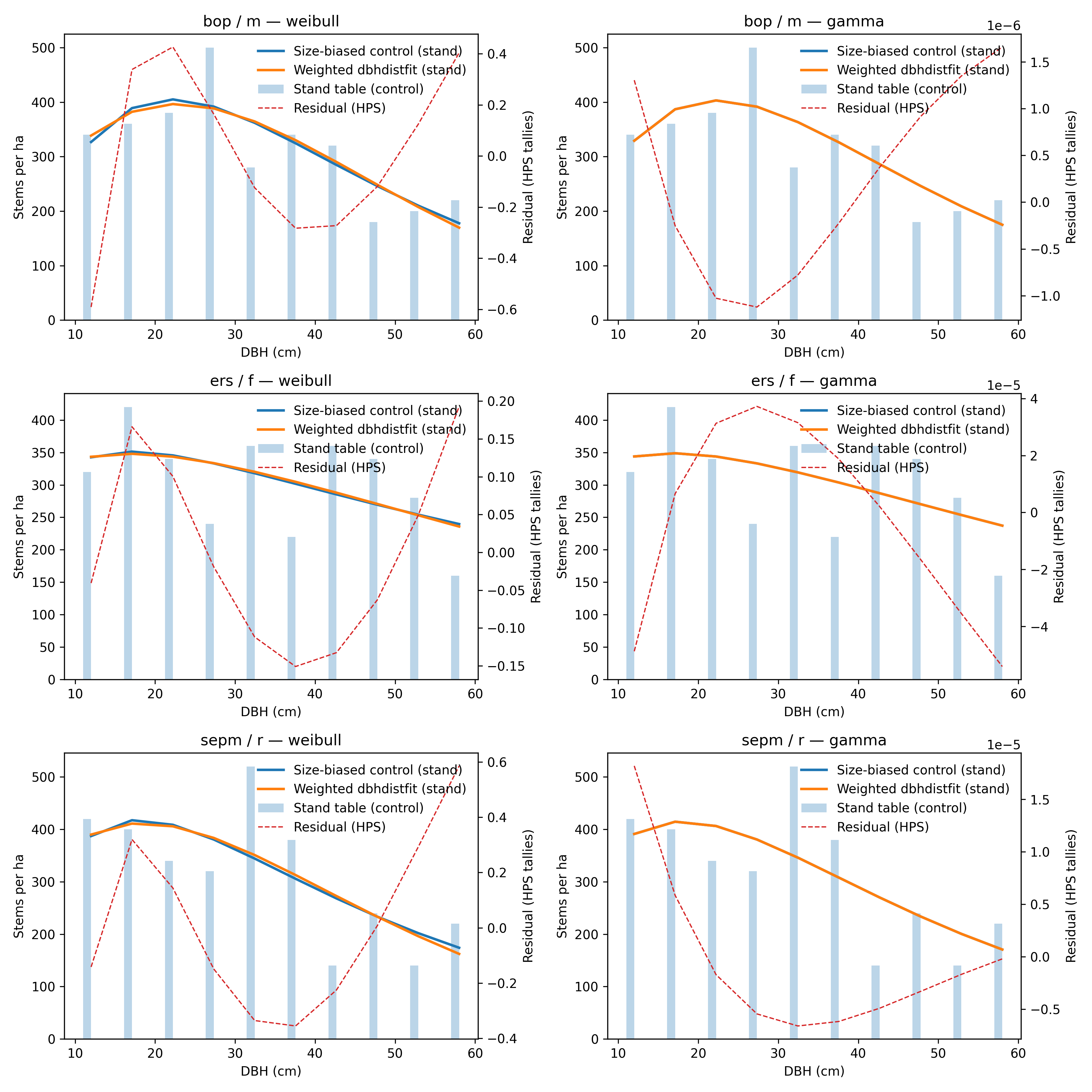
Figure 1 — Size-biased control vs. weighted nemora curves for the manuscript meta-plots. The dashed line shows residuals on the HPS tally scale.

Censored / Two-Stage Baseline

The reference notebook also aggregates the manuscript dataset into a censored meta-plot (DBH ≥ 20 cm) and fits the two-stage workflow via fit_censored_inventory. The exported table (docs/_static/reference_hps_censored_table.csv) records RSS, AICc, chi-square, and parameter values for each candidate distribution.

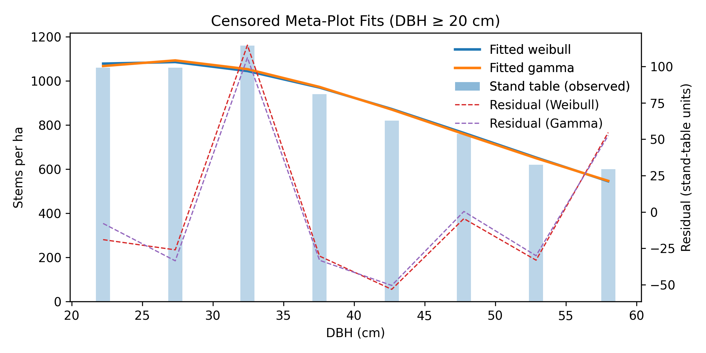
Figure 2 — Censored (DBH ≥ 20 cm) stand-table data with fitted Weibull and Gamma curves using the two-stage workflow. Residual lines highlight the agreement on the truncated support.

Diagnostics

• Inspect result.diagnostics["residuals"] for shape or bias.

• Compare result.gof metrics (RSS, AICc when available) across candidates.

• Plot the empirical stand table alongside fitted curves to confirm agreement with the manuscript workflow.

Next Steps

• Expose distribution filters and parameter previews in the CLI.

• Add worked examples for censored inventories and DataLad-backed datasets.

• Integrate notebook tutorials mirroring the published reproducibility bundles.

• Expand FAIR dataset coverage (see HPS dataset guide) with additional PSP plots and censored variants to support end-to-end parity tests.

.. todo:: Update this section once the nemora.ingest / sampling / synthesis modules land to reflect the broader workflow.